HNSW
On this page
Level: Advanced · Reading time: 9 min · Phase: 1 — RAG Foundations
In one line: HNSW (Hierarchical Navigable Small World) is a graph-based index that finds approximate nearest neighbours by hopping from point to closer point, starting on sparse "express" layers and finishing on a dense bottom layer.
Before you start: Vector Databases and Cosine Similarity. You should know what nearest neighbour search is, and that brute force checks every vector.
Explain it like I'm new
Think about travelling from a small village to a friend's house in another country. You do not walk street by street. You drive to a highway, take a flight to the right country, a train to the right city, then walk the last few streets. Each level is coarser and faster than the one below it.
Words to know:
- Index: a data structure that speeds up search by avoiding a full scan.
- ANN: Approximate Nearest Neighbour search, fast but may miss a true best match.
- Graph, node, edge: points joined by links; a node is a point (here, a vector) and an edge is a link.
- Greedy walk: always step to the neighbour that is closest to the query.
- Recall: the share of the true best matches the search actually finds.
- Query: the question, turned into a vector.
HNSW organizes vectors the same way.
- Every vector is a node in a graph. A graph is a set of points connected by links (edges).
- Each node is linked to some of its nearest neighbours.
- A few nodes also appear on higher layers with fewer nodes and longer links: the "highways" and "flights".
Search starts at the top layer, greedily moves to whichever neighbour is closest to the query, drops down a layer, and repeats. On the bottom layer, which contains every vector, it does a careful local search and returns the best k.
"Small world" refers to networks where any two nodes are connected by a short chain of links, like the "six degrees of separation" idea for people. "Navigable" means a simple greedy walk can find that short chain.
HNSW is one of the most widely used ANN indexes. It is available in FAISS, hnswlib, pgvector, Qdrant, Weaviate, Milvus, Elasticsearch/OpenSearch and others.
Watch it
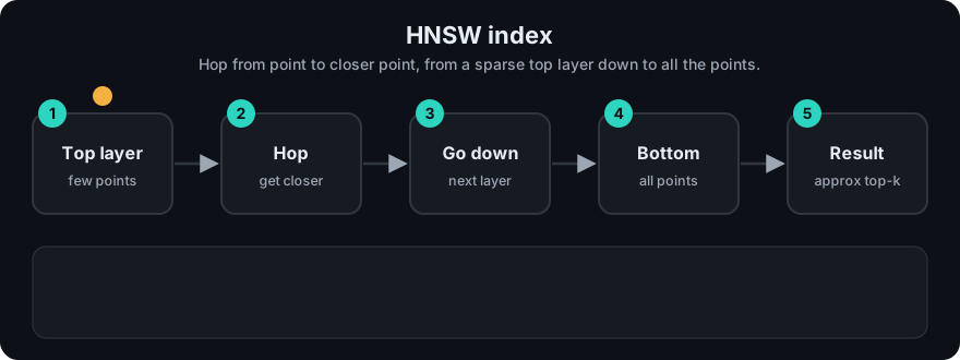
It plays on a loop. Read the caption in the box, one step at a time. Want to go at your own pace? Step through it with Previous and Next.
How it works
Building (insert one vector at a time)
- Pick a random top layer for the new node. Most nodes only live on layer 0; each higher layer has exponentially fewer nodes.
- Starting from the global entry point at the top, greedily walk down to the new node's top layer.
- On each layer from there down to 0, find nearby nodes (keeping a candidate list of size
ef_construction) and link the new node to up toMof them. Links go both ways.
Searching
- Start at the entry point on the top layer.
- Greedy step: move to any neighbour closer to the query; stop when no neighbour is closer. Go down one layer.
- On layer 0, run a beam search: keep the
ef(oref_search) best candidates found so far, expand their neighbours, stop when no candidate can improve the list. - Return the top k from that list.
Layer 2:  A ---------------------------- B              (few nodes, long links)
          |                              |
Layer 1:  A -------- C --------- D ----- B              (more nodes)
          |          |           |       |
Layer 0:  A - e - f - C - g - h - D - i - B - j - k     (all nodes, short links)
                                    ^ query lands near here
search: start A (L2) -> B is closer? yes -> drop to L1 -> D closer -> drop to L0 -> beam search around D
Key parameters
| Parameter | Meaning | Higher value means |
|---|---|---|
M | Links per node | Better recall, more memory, slower build |
ef_construction | Candidate list size when building | Better graph, slower build |
ef / ef_search | Candidate list size when searching | Better recall, slower queries |
Worked example
The repo demo uses 200 vectors and 50 queries. Brute force compares each query with all 200 vectors (recall@1 = 1.00, 200 computations). The graph index (one layer, same beam search) does this:
ef=2: about 43 distance computations per query, but recall@1 is only 0.88.ef=8: about 63 computations, recall@1 0.98.ef=32: about 127 computations, recall@1 1.00.
(recall@1 = how often the single best result is the true nearest vector.) So a small ef is cheap but misses more often. Raising ef buys accuracy with more work, still less than the 200 of brute force.
Code example
Real HNSW is too long for a lesson. code/rag_hnsw_ivf.py builds a single-layer navigable graph (each node linked to its nearest neighbours plus a few random long links) and searches it with the same beam search HNSW uses on layer 0. It counts distance computations so you can compare with brute force.
from rag_hnsw_ivf import GraphIndex, brute_force_search, make_clustered_data

data = make_clustered_data()                 # 200 2-D points in 4 clusters
graph = GraphIndex(data, m=5, random_links=2)
q = [9.5, 0.3]
print(brute_force_search(q, data, k=1))      # ([id], 200 distance computations)
print(graph.search(q, k=1, ef=8))            # usually same id, far fewer computations
Run python rag_hnsw_ivf.py to see recall@1 and average work for ef = 2, 8, 32. A bigger ef raises recall and costs more distance computations — the same knob as real HNSW.
In real projects (pip install hnswlib numpy):
import hnswlib
import numpy as np

dim, n = 384, 10_000
data = np.random.rand(n, dim).astype("float32")
index = hnswlib.Index(space="cosine", dim=dim)
index.init_index(max_elements=n, M=16, ef_construction=200)
index.add_items(data, np.arange(n))
index.set_ef(50)                                  # ef_search; must be >= k
labels, distances = index.knn_query(data[:3], k=5)
FAISS equivalent: faiss.IndexHNSWFlat(dim, 32).
When to use it / when not to
- Strong default for low-latency search with high recall on up to many millions of vectors that fit in RAM.
- Supports adding vectors one by one without retraining (unlike IVF, which needs a training step).
- Memory-heavy: it stores the vectors plus the links. For billions of vectors, IVF with compression or disk-based indexes may fit better.
- Deletes are harder; many systems mark items deleted and rebuild later.
| Flat (brute force) | HNSW | IVF | |
|---|---|---|---|
| Recall | Exact | High, tunable with ef | Tunable with nprobe |
| Query speed | Slow at scale | Very fast | Fast |
| Memory | Vectors only | Vectors + graph | Vectors + centroids |
| Build | None | Slower | Needs training (k-means) |
Common mistakes
- Leaving
ef_searchat a small default and losing recall without noticing. Measure recall against brute force on a sample. - Setting
eflower thank. - Very selective metadata filters on top of HNSW can break graph connectivity and hurt recall; check how your database handles filtered search.
- Expecting exact results. HNSW is approximate.
Recap
If you remember only three things:
- HNSW is a layered graph: sparse upper layers give long jumps, and the bottom layer holds every vector.
- Search walks greedily down the layers, then runs a beam search on the bottom layer.
ef_searchtrades recall for speed, so measure recall against brute force.
Interview questions
1. Explain HNSW in two sentences. <details><summary>Answer</summary> It builds a multi-layer proximity graph where upper layers are sparse with long links and the bottom layer has all vectors. Search greedily descends from the top layer and finishes with a beam search on the bottom layer. </details>
2. What do M and ef_search control? <details><summary>Answer</summary> M is the number of links per node (recall and memory). ef_search is the size of the candidate list during search (recall versus query latency). </details>
3. HNSW or IVF for 5 million vectors with strict latency needs? <details><summary>Answer</summary> HNSW is usually the first choice if memory allows, because it gives high recall at low latency without training. Choose IVF (often with quantization) when memory is the tighter limit. </details>
Go deeper
- Malkov & Yashunin, Efficient and robust approximate nearest neighbor search using Hierarchical Navigable Small World graphs — https://arxiv.org/abs/1603.09320
- hnswlib — https://github.com/nmslib/hnswlib
- FAISS docs — https://faiss.ai/
Prev: Dot Product · Next: IVF Index · Back to phase: Phase 1