01Why State Space Models Are the Most Important Architecture You’re Not Using
Every AI system you interact with today — GPT, Claude, Gemini — runs on Transformer architecture. Transformers are brilliant for what they do: they can attend to any token in context at once, making them powerful reasoners. But they carry a fundamental physical cost. Every new token generated must compare itself against every previous token. Double the context window, quadruple the compute. This is why running a 100,000-token context window costs so much money — and why truly long-context inference remains a solved-in-theory, broken-in-practice problem.
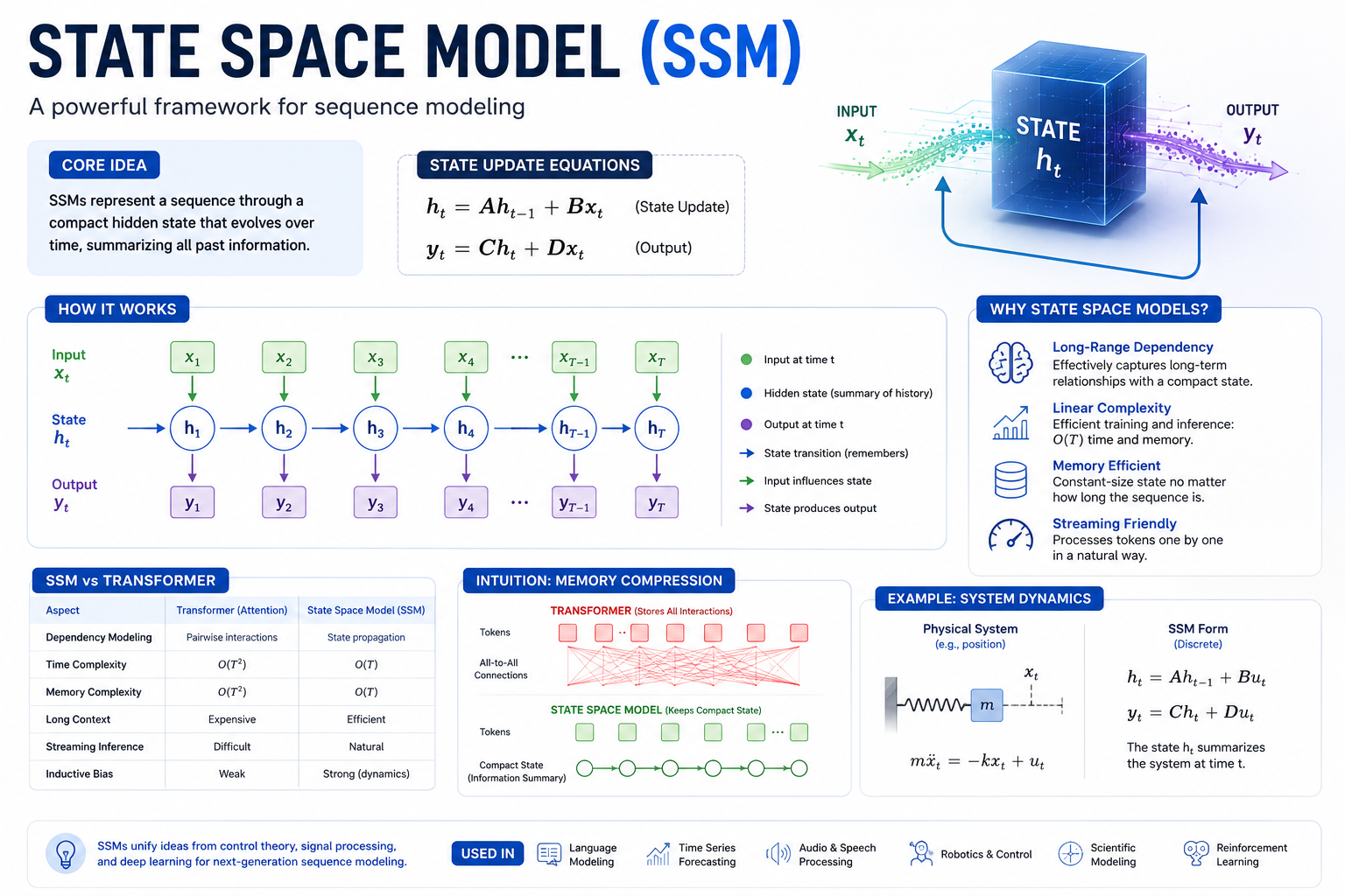
State Space Models (SSMs) take a completely different approach. Instead of remembering the whole past, they compress it. At every step, an SSM updates a fixed-size hidden state — a compact summary of everything that came before — and uses that to produce the next output. The past is not forgotten; it is continuously distilled. This single architectural decision gives SSMs O(n) compute and O(1) memory at inference — properties that no Transformer can match.
This guide explains exactly how that works: the math, the matrices, the tricks that make it trainable at scale, why the selective variant (Mamba) was the breakthrough that made SSMs competitive with Transformers on real language tasks, and where the field stands in 2026 with Mamba 3.
02The Core Equations — What an SSM Actually Computes
Definition — State Space Model: A mathematical system that models how hidden internal state h(t) evolves over time in response to an input x(t), and how that state produces an observable output y(t). Originated in control engineering (Kalman filtering, 1960s), adapted for deep learning sequences in 2021.
An SSM is defined by two equations. That’s it. Everything — the entire architecture, every variant from S4 to Mamba 3 — is ultimately a rethinking of these two lines of math:
The first equation says: the new hidden state is the old hidden state transformed by A, plus the new input scaled by B. The second says: the output is the hidden state read through C, plus a direct skip connection through D. Every token processed updates h(t). The history of all previous tokens lives — compressed — inside h(t).
The hidden state (purple) is a smoothed, compressed version of the input history — it never grows in size, regardless of sequence length.
The key insight: h(t) has a fixed size N, regardless of how long the sequence is. A 10-token sequence and a 1,000,000-token sequence produce the same size hidden state. Compare this to a Transformer’s KV cache, which grows by one entry per token, forever. This is the root of every efficiency advantage SSMs have.
03The Four Matrices — A, B, C, D Decoded
Everything an SSM learns lives in four matrices. Understanding what each one does intuitively is essential for understanding why SSM variants make the specific changes they do.
| Matrix | Shape | Role | What happens if it’s wrong? |
|---|---|---|---|
| A | N × N |
State dynamics — how memory evolves | Unstable training: exploding or vanishing gradients |
| B | N × 1 |
Input→state projection | New tokens fail to influence the hidden state |
| C | 1 × N |
State→output projection | Rich hidden state but meaningless output |
| D | 1 × 1 |
Direct input skip connection | Usually zero — low sensitivity, safe to remove |
The most critical matrix is A. If its eigenvalues are too large, the hidden state explodes. If too small, it forgets everything immediately. Getting A right — initializing it to have the right eigenvalue structure — is the core problem that HiPPO and S4 solved. In Mamba, A is diagonal (only N values stored, not N²), and B, C become input-dependent — the key to selectivity.
04Discretization — Bridging Continuous Math and Discrete Tokens
Definition — Discretization: The process of converting a continuous-time differential equation (h'(t) = Ah + Bx) into a discrete-time recurrence (h[k] = Āh[k-1] + B̄x[k]) suitable for processing sequences of tokens. The parameter Δ (delta) controls the time step size and is a learned parameter in Mamba.
Tokens are discrete. The SSM equations are continuous. This gap is bridged by discretization — converting the differential equation into a difference equation that steps forward one token at a time. The most common method is the Zero-Order Hold (ZOH):
The parameter Δ (delta) is especially important in Mamba. It controls how much the model “focuses” on the current token vs relying on existing memory. A large Δ means the current input dominates; a small Δ means memory persists strongly. Making Δ input-dependent is what enables selective attention without the quadratic cost of Transformer attention.
05The Duality: Recurrent at Inference, Convolutional at Training
One of the most important — and least understood — properties of SSMs is that the same model can be computed two ways, and the optimal choice depends on the context:
RECURRENT MODE
Process one token at a time. Each step: update h[k] using the previous h[k-1]. Requires only the last hidden state — O(1) memory. Cannot be parallelized (each step depends on previous).
CONVOLUTIONAL MODE
Unroll the recurrence into a convolution kernel K̄. Apply K̄ to the full input via FFT. The entire sequence is processed in parallel — O(n log n) compute. Enables GPU utilization.
This duality is the secret sauce of S4 and all subsequent SSMs. During training, the entire input sequence is known, so the model unfolds as a convolution and processes everything in parallel on GPU — matching Transformer training throughput. During inference, tokens arrive one at a time, so the model runs as a recurrence — O(1) memory, no KV cache growth, constant latency regardless of sequence length.
06HiPPO: The Memory Initialization That Made SSMs Work
Definition — HiPPO (High-order Polynomial Projection Operators): A mathematically optimal initialization scheme for the A matrix that compresses input history into Legendre polynomial coefficients. Introduced by Gu et al. (2020), HiPPO changed the SSM A matrix from “random guess” to “principled memory” — jumping performance on sequential MNIST from 60% to 98% accuracy overnight.
The original problem with SSMs was simple: how do you initialize matrix A so it doesn’t cause vanishing or exploding gradients while also capturing long-range dependencies? Random initialization fails. Even well-conditioned random matrices lose track of inputs from hundreds of steps ago.
HiPPO solves this by grounding A in mathematics. The idea: represent the history of inputs as a projection onto orthogonal polynomial bases (Legendre polynomials). The A matrix is then derived analytically to maintain this projection optimally. The result is a hidden state that is provably a compressed, lossless representation of the recent input history — not just a hopeful approximation.
Each bar represents a Legendre coefficient — together they encode the full recent input history. Watch the state update as new tokens arrive:
- HiPPO-LegS: uniform coverage — equal attention to all past inputs
- HiPPO-LagT: exponentially decaying attention — recent tokens weighted more
- S4 uses HiPPO-LegS with diagonal-plus-low-rank (DPLR) parameterization for efficient computation
- Mamba simplifies to pure diagonal A (just storing N numbers, not N×N) while preserving the HiPPO spirit
- Mamba 3 extends this with complex-valued diagonal A — recovering oscillatory dynamics that real-valued diagonals can’t capture
07S4: The Model That Proved SSMs Could Scale
The Structured State Space for Sequences (S4) model, published by Gu, Goel, and Ré in 2021, was the first SSM to match or beat Transformers on a diverse benchmark suite (Long Range Arena). It did this through three specific innovations stacked on top of HiPPO:
S4 achieved state-of-the-art on the Path-X benchmark (sequence length 16,384), demonstrated that 100,000+ token sequences were tractable, and inspired a generation of follow-on work: DSS, S4D, S5, H3, Hyena — each simplifying or extending the core architecture in different ways before Mamba made the next leap.
08Selective Scanning: How Mamba Made SSMs Context-Aware
Definition — Selective State Space Model (S6): An SSM where the B, C, and Δ matrices are functions of the current input token — not fixed learned parameters. This allows the model to dynamically choose what to remember and what to ignore, overcoming the linear time-invariant (LTI) limitation of S4. Called “selective scan” or “S6” in the Mamba paper.
S4 and all LTI SSMs share a critical weakness: the A, B, C matrices are fixed for every token. The model applies the same transformation to “the” as it does to “Transformer” as it does to “quantum”. It has no way to say “this token matters more than that one.” The state updates mechanically, equally, regardless of content.
This is exactly what Transformers do well: via attention weights, they can focus on specific past tokens. Mamba’s core innovation is recovering this capability without the quadratic cost, by making B, C, and Δ functions of the current input:
Bright tokens: Δ is large — this token dominates the state update (like attending). Dim tokens: Δ is small — previous memory persists strongly (like forgetting). This happens per-token, per-channel, in parallel.
The cost of making B, C, Δ input-dependent is that the convolutional representation no longer applies — you cannot precompute a fixed kernel if the kernel changes every step. Mamba solves this with a hardware-aware parallel scan algorithm: a custom CUDA kernel that computes the selective recurrence in parallel using prefix scan operations, achieving S4-like training throughput without the fixed-kernel shortcut.
- A remains diagonal and fixed (not input-dependent) — preserving stable gradients
- B, C, Δ are all projected from the current token via small linear layers
- Large Δ ≈ “pay attention to this token” (discretization zooms in)
- Small Δ ≈ “ignore this token, preserve state” (discretization steps slowly)
- This is mathematically equivalent to soft, content-based gating — without attention heads, without O(n²) cost
09SSM vs Transformer — A Precise Comparison
| Property | Transformer | SSM (S4/Mamba) | LSTM/RNN |
|---|---|---|---|
| Training complexity | O(n²) attention | O(n log n) convolution | O(n) but sequential |
| Inference memory | O(n) KV cache — grows forever | O(1) fixed hidden state | O(1) hidden state |
| Inference speed per token | Slows down as context grows | Constant regardless of context | Constant |
| Long-range dependencies | Excellent (direct attention) | Strong (HiPPO + selective) | Weak (vanishing gradient) |
| Random access retrieval | Strong — direct key-value lookup | Moderate — compressed state | Poor |
| Streaming input | Expensive — re-attends all past | Native — state update per token | Native |
| Parallelism (training) | Fully parallel | Parallel scan (hardware kernel) | Sequential only |
| State compression | None — stores all tokens in KV | Aggressive — fixed N dimensions | Partial — gating mechanism |
| Theoretical grounding | Empirical (attention is useful) | Control theory + HiPPO mathematics | Heuristic gating |
10The SSM Family Tree — From S4 to Mamba 3
11Real-World Use Cases — Where SSMs Win
| Domain | Why SSM excels | Specific advantage |
|---|---|---|
| Long-document Q&A | 100K+ token contexts fit in fixed memory | No KV cache explosion — constant latency |
| Real-time audio/speech | Streaming token-by-token O(1) | Live transcription without buffer delays |
| Time-series forecasting | Continuous dynamics modeled natively | Better than Transformers on irregular intervals |
| Genomics / DNA sequences | Sequences millions of tokens long | Transformer is physically impossible; SSM scales |
| Agentic AI pipelines | 100s of agents × constant memory = feasible | Predictable memory per agent regardless of steps |
| Edge / mobile AI | Constant RAM — no growth at runtime | Fits on device without managed KV cache |
| RAG retrieval encoding | Fixed-size embedding regardless of chunk length | Consistent vector dimensions for any document size |
- Use SSMs when your sequences exceed 8K–16K tokens — Transformer KV cache becomes the bottleneck here
- Prefer Transformers for tasks requiring precise retrieval of specific facts from a fixed-length context — SSM compression can lose exact token positions
- Hybrid architectures (alternating SSM and attention layers) often give best-of-both results — consider this for general-purpose LLMs
- For streaming inference (voice assistants, live analysis), SSM is the only architecture that maintains constant latency regardless of session length
- In RAG pipelines, SSM-encoded embeddings have the advantage of fixed size regardless of input length — simplifying indexing
12FAQ — Every Real Question About State Space Models Answered
Fact A State Space Model (SSM) is a sequence processing framework that maintains a fixed-size hidden state — a compact summary of all past inputs — and updates it one token at a time using matrix multiplications.
Think of it like a person with perfect short-term working memory but a fixed number of “memory slots.” Every new input updates those slots — more important things can overwrite less important things (in selective SSMs like Mamba). Unlike a Transformer, which stores the full conversation history in a growing KV cache, an SSM always uses the same amount of memory no matter how long the sequence. The tradeoff: if something important was long ago and has been gradually overwritten, it may no longer be recoverable — this is why SSMs historically struggled with exact retrieval tasks, though Mamba and Mamba 3 have largely addressed this with selective updating.
Fact In the SSM equations h'(t) = Ah + Bx and y = Ch + Dx: A controls how the hidden state evolves on its own (memory dynamics), B projects input into the state space, C projects the state back to output space, and D is a direct skip connection from input to output.
A is the most critical. Its eigenvalues determine stability: eigenvalues with negative real parts cause the state to decay (forget), while values near the imaginary axis create oscillatory memory (useful for periodic signals). The HiPPO initialization sets A to the mathematically optimal structure for remembering polynomial projections of input history. B and C are input-output projections that are fixed in LTI SSMs (S4) but become input-dependent in Mamba — this is the core of selective scanning. D is usually set to zero or one and adds a residual path similar to skip connections in ResNets.
Fact Δ (delta) is the time-step parameter that bridges continuous SSM theory and discrete token sequences. In Mamba, Δ is made input-dependent, acting as a content-based gating mechanism: large Δ means “absorb this token strongly into state,” small Δ means “let existing state persist, barely update.”
This is a profound insight. The discretization parameter, usually treated as a fixed hyperparameter in S4, becomes the model’s attention mechanism in Mamba — without any of the quadratic cost. When a token has large Δ, the discretized A approaches the identity matrix (Ā ≈ I), meaning the state is almost reset to the new input. When Δ is small, Ā ≈ A (original dynamics dominate), meaning memory is retained. Making Δ = Softplus(Linear(x)) gives the model full control over when to remember and when to update — per token, per dimension, per channel — all in O(n) time.
Fact Pure SSMs match or exceed Transformers on most language modeling benchmarks at 1B–3B scale, but Transformers retain advantages in tasks requiring precise random-access retrieval of specific tokens from a fixed known context — such as certain in-context learning and multi-hop reasoning tasks.
The current research consensus (2026) points toward hybrid architectures — models that alternate SSM layers with occasional attention layers — as the optimal design for general-purpose language models. Pure SSMs are the right choice for deployment-constrained scenarios: streaming inference, long contexts, edge devices, and agentic pipelines where O(1) memory is a hard requirement. Transformers remain superior for tasks that resemble database lookup (retrieving a specific fact verbatim from a known passage). The two architectures are complements, not pure substitutes.
Fact S4 (2021) is a linear time-invariant SSM with fixed A/B/C matrices and HiPPO initialization. Mamba (2023) adds input-dependent B, C, Δ (selective scanning). Mamba 3 (ICLR 2026) adds complex-valued A, exponential-trapezoidal discretization, and MIMO formulation — together achieving +1.8pp accuracy over the prior best SSM with 50% smaller state.
The progression tracks increasing expressiveness at each step: S4 proves SSMs can train efficiently at scale via the convolutional representation. Mamba proves they can be context-aware via selective scanning. Mamba 2 unifies SSMs and linear attention into a single theoretical framework (State Space Duality). Mamba 3 shifts the design philosophy from training efficiency to inference efficiency — asking not “how do we train this on GPU?” but “how do we deploy this with the best quality-per-compute ratio?” The three innovations of Mamba 3 (complex A, new discretization, MIMO) work together to improve the quality-efficiency Pareto frontier without increasing inference latency.
Fact HiPPO (High-order Polynomial Projection Operators) is a mathematically derived initialization for the SSM A matrix, constructed so that the hidden state always represents the optimal polynomial approximation of the input history. It was introduced by Gu et al. in 2020 and improved sequential MNIST accuracy from 60% to 98% without any other architectural change.
Without HiPPO, the A matrix must be randomly initialized — and random matrices either cause the hidden state to explode (eigenvalues > 1) or instantly forget everything (eigenvalues << 1). HiPPO solves this by grounding A in the mathematics of approximation theory: specifically, the problem of compressing a function into its Legendre polynomial coefficients updates exactly as the HiPPO-LegS matrix specifies. This means the hidden state is provably the best possible fixed-size representation of the input history — not just a heuristic. S4 uses HiPPO-LegS with DPLR structure. Mamba simplifies to diagonal A but retains the HiPPO spirit of spectral initialization. Mamba 3 extends this with complex-valued diagonal entries, recovering richer dynamics.
Fact SSMs encode positional information implicitly through the recurrence structure — each token is processed in order and the hidden state carries temporal context naturally, unlike Transformers where position is injected explicitly (sinusoidal, RoPE, ALiBi) because attention is permutation-equivariant without it.
Because the state update h[k] = Āh[k-1] + B̄x[k] processes tokens sequentially and the previous state h[k-1] depends on all prior tokens in order, the model inherently knows where it is in the sequence. Token 5’s representation in the hidden state is different from token 500’s even if the input token is identical — because the state it was added into was different. This means SSMs get position for free from the recurrent structure, without adding sinusoidal encodings, rotary embeddings, or any other positional machinery. In practice, SSMs may still benefit from relative position encodings for very long sequences, but the baseline position encoding requirement is lower than for Transformers.
Fact SSM inference (the recurrent mode) has much higher arithmetic intensity than Transformer KV-cache attention — meaning more useful math operations per byte of memory transferred. On ARM chips (Apple Silicon, AWS Graviton, Qualcomm), memory bandwidth is the bottleneck, so higher arithmetic intensity directly translates to faster throughput.
Transformer decoding is memory-bandwidth-bound: for each new token, the entire KV cache must be loaded from memory to compute attention scores — O(n) memory reads per token. SSM decoding is compute-bound: only the fixed-size hidden state (N parameters) is needed per step, and the matrix multiply Āh + B̄x keeps the ALUs busy. Modern SIMD instruction sets (NEON on ARM, AVX-512 on x86) are designed for exactly this kind of dense small-matrix math. This is also why TurboVec’s nibble-split lookup table maps perfectly to NEON — both TurboVec and Mamba inference are structured to maximize SIMD utilization on the same hardware.
13Where SSMs Go From Here
State Space Models began as a niche idea from control engineering, became a serious Transformer alternative with S4, crossed the quality threshold with Mamba’s selective scanning, and in 2026 stand as the most principled, theoretically grounded architecture for inference-efficient AI. The journey from the HiPPO matrix’s 60%→98% accuracy jump to Mamba 3’s 1.8pp advance over Gated DeltaNet is a story of mathematics steadily winning over heuristics.
The next frontier is clear: hybrid architectures that combine SSM layers’ O(1) inference memory with occasional attention layers’ retrieval precision; multi-modal SSMs that apply the same recurrent efficiency to vision, audio, and genomics simultaneously; and on-device inference where the constant-memory property finally makes truly local, private AI tractable on laptops and phones.
If you are building AI systems today — RAG pipelines, agentic workflows, real-time analysis, or long-context applications — understanding State Space Models is no longer optional. They are the architecture that defines what comes after the Transformer era.
Related reading: Mamba 3 vs Transformer Deep Dive · TurboVec & Google TurboQuant Guide · RAG Pipeline Implementation
Master the Architecture Replacing Transformers
Get our SSM implementation notebooks, Mamba 3 benchmarking scripts, and the complete sequence model comparison guide — free.
🚀 Get the Free Guides