Why Attention Changed Everything in 2017
Before 2017, sequence modeling meant LSTMs, GRUs, and recurrent networks. They processed tokens one at a time, left to right, compressing all context into a single hidden state vector. When the sentence was 50 tokens long and a crucial word was at position 3, the model had to chain information through 47 intermediate states without losing it. Gradient signals weakened exponentially over distance. Long-range dependencies were the Achilles heel of every recurrent model.
The paper “Attention Is All You Need” (Vaswani et al., 2017) replaced this bottleneck with a single, beautiful idea: let every token attend directly to every other token simultaneously. No recurrence. No chained state propagation. Every position in the sequence can directly query every other position in one matrix multiplication. The result was not just faster training — it was qualitatively different reasoning. GPT, BERT, T5, LLaMA, Claude — every major language model of the last eight years is built on this mechanism.
What Query, Key, and Value Actually Mean
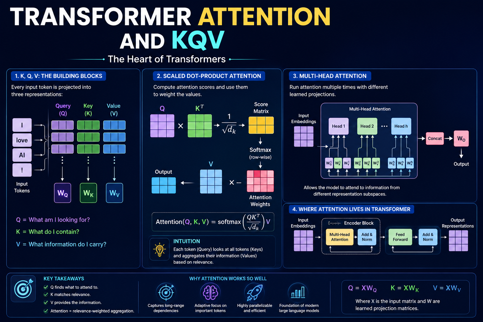
Definition — Self-Attention: A mechanism where each token in a sequence learns to represent itself as a Query (what am I looking for?), a Key (what do I advertise about myself?), and a Value (what information do I pass if I match?). Attention weights are computed by matching Queries against all Keys, then using those weights to aggregate the corresponding Values.
The Q/K/V naming comes from database retrieval — but understanding the intuition matters more than the analogy. Here is the clearest way to think about it:
- Query (Q): The current token asking a question. “I am the word it — who in this sentence am I referring to?” The Query is a projection of the current token that encodes what it’s searching for.
- Key (K): What every token broadcasts about itself. “I am bank — I have features relevant to finance OR geography.” Each token’s Key is a projection of itself that answers the question “can I help this query?”
- Value (V): The actual information payload. If the Query-Key match is high, the Value is the information that gets delivered. The Key opens the door; the Value is what’s behind it.
All three — Q, K, V — are computed by multiplying the same input embedding by three separate learned weight matrices: W_Q, W_K, W_V. These matrices are the only parameters the attention mechanism learns. The attention score between any two tokens is the dot product of the Query of one against the Key of the other — a scalar that measures how relevant token B is to token A’s question.
Interactive Transformer Attention Visualizer
Click any token below to set it as the Query. Watch how attention scores are computed against all Keys, softmax normalizes them into weights, and the weighted Values are aggregated into the output. Step through each stage of the computation.
The Attention Equation — Every Part Decoded
Definition — Scaled Dot-Product Attention: The core attention operation: Attention(Q,K,V) = softmax(QKT / √dk) · V. Takes Query, Key, Value matrices as input; outputs a context-enriched representation where each token’s representation is a weighted sum of all Values, weighted by query-key compatibility.
Let’s take each part of the formula apart and understand why it exists:
Part 1: QKT — The Compatibility Matrix
Multiplying Q (shape: seq_len × d_k) by KT (shape: d_k × seq_len) produces a square matrix of shape seq_len × seq_len. Entry [i,j] in this matrix is the dot product of token i’s query with token j’s key — a single number measuring how compatible token i’s question is with token j’s advertisement. Higher = more relevant.
Part 2: / √dk — The Stability Scaling
Without scaling, as dimension d_k grows, the dot products grow proportionally in magnitude. Large dot products push the softmax function into regions with extremely small gradients — the “softmax saturation” problem. Dividing by √d_k keeps the variance of the dot products at 1.0 regardless of d_k, preventing this. This is why the denominator is √d_k and not, say, d_k itself.
Part 3: softmax(·) — Converting Scores to Weights
Softmax converts the raw scores to a probability distribution that sums to 1.0. Each entry now represents “what fraction of my attention should go to token j?” Sharp distributions mean focused attention on a few tokens. Flat distributions mean diffuse attention across many tokens. Temperature (scale factor) controls this sharpness.
Part 4: · V — The Weighted Sum
Finally, multiply attention weights (seq_len × seq_len) by V (seq_len × d_v). This is a weighted sum: for each position i, sum up all Value vectors weighted by how much attention position i paid to each key. The result is a new representation of each token that incorporates information from all relevant context positions.
Multi-Head Attention — Parallel Viewpoints
Definition — Multi-Head Attention: Running h independent attention operations in parallel, each using different learned projections (W_Q^i, W_K^i, W_V^i). Each head can specialize in different linguistic patterns — syntax, coreference, positional proximity. Outputs are concatenated and projected: MultiHead(Q,K,V) = Concat(head_1,…,head_h) · W_O.
Single-head attention forces the model to represent all semantic relationships in one subspace. Multi-head attention solves this by running h independent attention operations in parallel, each operating in a d_k = d_model/h dimensional subspace. Each head develops its own W_Q, W_K, W_V matrices and attends to different patterns.
- Head specialization: In trained language models, different heads consistently take on different roles — some track syntactic dependencies (subject-verb), others handle coreference resolution (pronoun-antecedent), others attend to local positional context
- No extra parameters vs single large head: If d_model = 512 and h = 8, each head uses d_k = 64. The total parameter count is the same as one 512-dim head, but expressiveness is dramatically higher
- Output projection W_O: Concatenated head outputs (seq_len × h·d_v) are projected back to d_model via W_O, mixing information across heads
- GPT-2 small uses 12 heads, d_model=768: Each head sees a 64-dimensional projection of each token’s embedding
Causal Masking — Why Decoders Can’t See the Future
Encoders (BERT) use bidirectional attention — every token can attend to every other token. But autoregressive decoders (GPT, LLaMA) must generate tokens one at a time, left to right. If token at position 5 could attend to token at position 6 during training, it would simply copy the answer from the future — the model would learn nothing useful.
Causal masking prevents this by setting the attention scores for future positions to −∞ before the softmax. After softmax, e^(−∞) = 0, so those positions contribute zero weight. Each token can only attend to positions at or before its own position. The attention matrix becomes lower-triangular.
| Architecture | Attention type | Masking | Examples |
|---|---|---|---|
| Encoder-only | Bidirectional self-attention | None — full context | BERT, RoBERTa, DeBERTa |
| Decoder-only | Causal self-attention | Causal mask (lower-triangular) | GPT-2/3/4, LLaMA, Claude, Gemini |
| Encoder-Decoder | Self + cross-attention | Causal in decoder; bidirectional in encoder | T5, BART, original Transformer |
Self-Attention vs RNN / LSTM vs Convolution
| Property | Self-Attention | RNN / LSTM | Convolution |
|---|---|---|---|
| Max path length | O(1) — direct token-to-token | O(n) — chains through all steps | O(n/kernel) — limited receptive field |
| Parallelism | Full (all tokens at once) | Sequential (one step at a time) | Full |
| Complexity per layer | O(n²·d) — quadratic in seq length | O(n·d²) — linear in seq length | O(k·n·d) — linear with small kernel |
| Long-range dependencies | Excellent — direct access | Poor — vanishing gradient | Limited by kernel size |
| Interpretability | Attention weights = explicit | Hidden state = opaque | Filter-based, limited |
| Memory at inference | O(n) KV cache grows | O(1) hidden state | O(k) kernel only |
PyTorch Implementation — Attention From Scratch
import torch
import torch.nn as nn
import torch.nn.functional as F
import math

class ScaledDotProductAttention(nn.Module):
    """
    Single-head scaled dot-product attention.
    Attention(Q, K, V) = softmax(QK^T / sqrt(d_k)) * V
    """
    def __init__(self, d_k: int, dropout: float = 0.1):
        super().__init__()
        self.d_k = d_k
        self.dropout = nn.Dropout(dropout)

    def forward(self, Q, K, V, mask=None):
        # Q: [batch, seq, d_k]  K: [batch, seq, d_k]  V: [batch, seq, d_v]

        # Step 1: Compute raw attention scores — QK^T
        scores = torch.matmul(Q, K.transpose(-2, -1))  # [batch, seq, seq]

        # Step 2: Scale by 1/sqrt(d_k) for gradient stability
        scores = scores / math.sqrt(self.d_k)

        # Step 3: Apply causal mask (decoder) — set future to -inf
        if mask is not None:
            scores = scores.masked_fill(mask == 0, float('-inf'))

        # Step 4: Softmax — convert scores to attention weights (sums to 1)
        weights = F.softmax(scores, dim=-1)          # [batch, seq, seq]
        weights = self.dropout(weights)               # regularization

        # Step 5: Weighted sum of Values
        output = torch.matmul(weights, V)             # [batch, seq, d_v]

        return output, weights  # weights for visualization


class MultiHeadAttention(nn.Module):
    """
    Multi-head attention: run h attention heads in parallel,
    each operating in d_model/h dimensional space.
    """
    def __init__(self, d_model: int, h: int, dropout: float = 0.1):
        super().__init__()
        assert d_model % h == 0, "d_model must be divisible by h"

        self.d_k = d_model // h
        self.h = h

        # Each head gets its own projection matrices
        self.W_Q = nn.Linear(d_model, d_model)  # [d_model -> h * d_k]
        self.W_K = nn.Linear(d_model, d_model)
        self.W_V = nn.Linear(d_model, d_model)
        self.W_O = nn.Linear(d_model, d_model)  # Output projection

        self.attention = ScaledDotProductAttention(self.d_k, dropout)

    def split_heads(self, x, batch_size):
        """Split last dim into (h, d_k) then transpose for attention."""
        x = x.view(batch_size, -1, self.h, self.d_k)
        return x.transpose(1, 2)  # [batch, h, seq, d_k]

    def forward(self, Q, K, V, mask=None):
        batch_size = Q.size(0)

        # Project Q, K, V and split into h heads
        Q = self.split_heads(self.W_Q(Q), batch_size)  # [batch, h, seq, d_k]
        K = self.split_heads(self.W_K(K), batch_size)
        V = self.split_heads(self.W_V(V), batch_size)

        # Scaled dot-product attention for all heads simultaneously
        x, attn_weights = self.attention(Q, K, V, mask)  # [batch, h, seq, d_k]

        # Concatenate heads and project back to d_model
        x = x.transpose(1, 2).contiguous()              # [batch, seq, h, d_k]
        x = x.view(batch_size, -1, self.h * self.d_k)   # [batch, seq, d_model]
        output = self.W_O(x)                             # [batch, seq, d_model]

        return output, attn_weights


# ── Usage example ──
d_model, h, seq_len, batch = 512, 8, 10, 2
mha = MultiHeadAttention(d_model=d_model, h=h)

# In self-attention: Q = K = V = same input
x = torch.randn(batch, seq_len, d_model)

# Causal mask: lower-triangular (decoder)
mask = torch.tril(torch.ones(seq_len, seq_len)).unsqueeze(0).unsqueeze(0)

output, weights = mha(x, x, x, mask=mask)
print(f"Output shape:  {output.shape}")   # [2, 10, 512]
print(f"Weights shape: {weights.shape}")  # [2, 8, 10, 10] — per head
# ── Flash Attention (2022) — Memory-efficient equivalent ──
# For production, use Flash Attention instead of naive implementation.
# Same mathematical output but O(n) memory via kernel fusion.

from torch.nn.functional import scaled_dot_product_attention

# PyTorch 2.0+ has Flash Attention built in:
output = scaled_dot_product_attention(
    Q, K, V,
    attn_mask=None,      # or causal mask
    dropout_p=0.1,
    is_causal=True,      # enables causal masking automatically
    scale=None           # defaults to 1/sqrt(d_k)
)
# Automatically uses Flash Attention on CUDA when available
# Memory: O(n) instead of O(n^2) — critical for long contexts
Best Practices Checklist for Attention in Production
- Always use Flash Attention (
torch.nn.functional.scaled_dot_product_attentionwithis_causal=True) in production — same output, O(n) memory instead of O(n²) - For sequences longer than 8,192 tokens, consider Sliding Window Attention (each token attends to only a local window + global tokens) as in Mistral — prevents memory explosion
- Use Rotary Position Embedding (RoPE) for position encoding in decoder-only models — outperforms absolute and sinusoidal encodings on long contexts and generalizes beyond training length
- When fine-tuning, apply LoRA (Low-Rank Adaptation) to W_Q and W_V matrices — empirically the most impactful weight matrices to adapt, with 10-100× parameter efficiency over full fine-tuning
- Monitor attention entropy during training — overly peaked attention distributions (entropy near 0) indicate head collapse; overly flat distributions suggest the head isn’t learning useful patterns
- For multi-head attention, prune heads that show redundant attention patterns after training — up to 20% of heads in GPT-2 can be pruned with negligible quality loss
- In multi-document RAG systems, use cross-document attention patterns to debug whether the model is actually retrieving the right context — visualize attention from the answer generation token back to the source
- Use Grouped-Query Attention (GQA) for inference efficiency — multiple query heads share a single key-value head, reducing KV cache size by 4-8× (used in LLaMA 3, Mistral)
Related reading: State Space Models Explained · Mamba 3 vs Transformer · RAG Pipeline Guide
FAQ — Every Transformer Attention Question Answered
Fact Q (Query), K (Key), and V (Value) are three linear projections of the input embedding, computed by multiplying the input by learned weight matrices W_Q, W_K, W_V respectively.
Intuitively: Query is what the current token is searching for (“I am ‘it’ — who am I referring to?”), Key is what each token advertises about itself (“I am ‘bank’ — relevant to finance/geography”), and Value is the information payload delivered when there is a match. The attention score between tokens i and j is the dot product of token i’s Query with token j’s Key, scaled and normalized. The output is a weighted sum of all Values weighted by these scores. All three matrices have the same dimension d_k (usually d_model / num_heads) and are the core learned parameters of each attention layer.
Fact Without the √d_k scaling, the dot products Q·K^T grow proportionally to d_k in magnitude, pushing softmax into saturation regions where gradients are near-zero — causing training instability and vanishing gradients.
Specifically: if Q and K both have components drawn from a unit normal distribution, their dot product has variance d_k. Dividing by √d_k normalizes this variance back to 1.0 regardless of dimension. This keeps softmax in its “sensitive” regime where gradients are healthy. The original Vaswani et al. 2017 paper noted that for small d_k this doesn’t matter much, but for larger dimensions (d_k = 64, 128) training becomes unstable without the scaling. This is also why the denominator is specifically √d_k — it’s the standard deviation normalization for a d_k-dimensional dot product.
Fact In self-attention, Q, K, and V all come from the same sequence — tokens attend to each other within one sequence. In cross-attention, Q comes from one sequence (the decoder’s current state) while K and V come from another sequence (the encoder’s output).
Self-attention is used in every transformer layer to let tokens contextualize each other. Cross-attention appears in encoder-decoder architectures (T5, BART, original transformer) to let the decoder query the encoder’s representations. For example, in machine translation, the decoder generating the French output token uses cross-attention to query the encoder’s representations of the English input — the decoder’s current partial output forms Q, while the English encoding forms K and V. In decoder-only models (GPT, LLaMA, Claude), there is no encoder, so all attention is self-attention with causal masking.
Fact Multi-head attention runs h independent attention operations in parallel, each using its own W_Q^i, W_K^i, W_V^i matrices in a d_k = d_model/h dimensional subspace. Outputs are concatenated and projected by W_O back to d_model.
The motivation: a single attention head must represent all semantic relationships (syntax, coreference, topic, position) in one subspace — a fundamental bottleneck. With h heads, each head can specialize in different patterns. In trained language models, head specialization is empirically observable: some heads consistently track syntactic dependency (subjects to verbs), others resolve coreference (pronouns to antecedents), others focus on local positional context. The total parameter count is the same as one large-d_k head, but the representational diversity is dramatically higher. GPT-2 uses 12 heads, GPT-3 uses 96 heads in its largest variant.
Fact Flash Attention (Dao et al., 2022) is a hardware-aware implementation of exact scaled dot-product attention that reduces memory complexity from O(n²) to O(n) by recomputing attention in fused GPU kernel passes instead of materializing the full n×n attention matrix.
Standard attention must write the n×n score matrix to GPU HBM (high-bandwidth memory) — for a 4,096-token sequence this is 16M floats per head per layer, quickly exhausting VRAM. Flash Attention computes attention in tiles that fit in on-chip SRAM (L2 cache), recomputing intermediate values during the backward pass instead of storing them. The output is mathematically identical to standard attention. Flash Attention 2 and 3 (2023–2024) add further optimizations for parallelism and hardware utilization. It is now the default implementation in PyTorch 2.0+, HuggingFace Transformers, and all major production LLM inference stacks.
Fact The KV cache stores the Key and Value matrices for all previously generated tokens so they don’t need to be recomputed at each new generation step. It grows by d_k + d_v floats per layer per new token.
During autoregressive generation, each new token must compute attention against all previous tokens. Without caching, this would require recomputing K and V for every past token at every step — O(n) recomputation per token. The KV cache trades memory for compute: store K and V for all past tokens, then each new step only computes the new token’s Q and attends it against the cached K, V. The downside is linear memory growth: a 100,000-token context with 32 layers, 32 heads, and d_k=128 requires ~3.3 GB of KV cache at float16. This is the primary memory bottleneck driving interest in SSMs (Mamba, Mamba 3) which replace the KV cache with a fixed-size hidden state.
Fact Attention is permutation-equivariant by design — the same output is produced regardless of token order because attention scores are based on content, not position. Positional encoding injects order information by adding a position-dependent signal to each token’s embedding before attention is computed.
Without positional encoding, “The cat sat on the mat” and “The mat sat on the cat” would produce identical attention outputs — clearly wrong. The original 2017 transformer used sinusoidal positional encodings. Modern models predominantly use Rotary Position Embedding (RoPE) — introduced in RoFormer (2021) and adopted by LLaMA, Mistral, Qwen, and most recent models. RoPE encodes position by rotating the Q and K vectors by a position-dependent angle before computing their dot product, so that the score naturally reflects relative distance between tokens. RoPE generalizes better to longer contexts than absolute encodings and is more hardware-efficient than ALiBi (Attention with Linear Biases).
Fact Grouped-Query Attention shares a single set of K and V heads across multiple Q heads — if there are 8 Q heads per group and 4 KV groups, the KV cache is 4× smaller than standard multi-head attention with no significant quality loss.
Standard multi-head attention with 32 heads requires 32 K-head cache entries and 32 V-head cache entries per token. GQA reduces this: multiple query heads share the same key-value pair. LLaMA 3 (8B model) uses 8 key-value heads shared across 32 query heads — a 4× KV cache reduction. Multi-Query Attention (MQA) is the extreme version: all query heads share a single K and V (used in Falcon). GQA is the balanced version that achieves most of MQA’s memory savings with negligible quality degradation, making it the current industry standard for production LLMs requiring fast inference at long contexts.
Conclusion — Attention Is Still the Core of Modern AI
From the “Attention Is All You Need” paper in 2017 to GPT-4, LLaMA 3, and Claude in 2026 — the fundamental mechanism has not changed. Every major language model still runs on the same core operation: multiply Q by K-transpose, scale, softmax, multiply by V. What has evolved is the engineering around it: Flash Attention made it memory-efficient, RoPE made position encoding robust, GQA made inference practical at scale, and multi-head attention made it semantically rich.
Understanding attention at the level of its equations — not just its intuition — is the prerequisite for understanding every architectural innovation in modern AI. When you understand why /√d_k exists, you understand gradient flow. When you understand why causal masking works, you understand autoregressive generation. When you understand KV cache growth, you understand why State Space Models like Mamba exist. The attention mechanism is the foundation that everything else is built on or built against.
Related reading: State Space Models: The Architecture After Transformers · Mamba 3 vs Transformer Deep Dive · TurboVec: Vector Search at Scale
Master the Full Transformer Stack
Get our interactive attention notebook, multi-head attention visualizer code, and the complete “Attention is All You Need” implementation guide — free.
🚀 Get the Free Guides